Math and Stats for ML (Deep)

Why This Matters

If you cannot reason from first principles, you will plateau quickly in ML engineering roles. Top product-company ML interviews and day-to-day decisions require you to explain why a model failed, why one metric matters more than another, and why one optimization strategy is safer under constraints.

Most people memorize formulas. Strong ML engineers use mathematical reasoning to reduce expensive trial-and-error cycles. This module is your foundation layer for everything else in the path.

Prerequisites

• High-school algebra (comfort with equations and rearrangement)
• Basic Python and NumPy
• Willingness to derive simple expressions by hand
• Curiosity to connect math decisions to product outcomes

Learning Outcomes

After this module, check that you can:

• Explain gradient-based learning behavior from loss curves and parameter updates
• Choose and defend evaluation metrics under business constraints
• Diagnose underfitting/overfitting using training dynamics
• Use probability and statistics to quantify confidence in model comparisons
• Connect regularization and optimization choices to real-world model robustness

Core Concepts

1) Linear Algebra for Representation

• Vectors as feature containers
• Matrices as batch and transformation operators
• Dot product as weighted evidence accumulation
• Norms as geometry of magnitude and distance

2) Probability for Uncertainty

• Random variables and expectation
• Conditional probability and Bayes intuition
• Distributions relevant to modeling assumptions
• Variance as uncertainty budget in decisions

3) Statistics for Model Decisions

• Sampling and estimation error
• Confidence intervals for model comparison
• Hypothesis testing limitations in product settings
• Effect size vs statistical significance

4) Optimization for Learning Dynamics

• Objective functions and loss surfaces
• Gradient descent variants and stability
• Learning-rate schedules
• Regularization as constrained optimization

Mental Models and Tradeoffs

Mental Model: "Metrics are product contracts"

A metric is not a leaderboard number. It encodes what failure you can tolerate. Optimizing the wrong metric is equivalent to implementing the wrong product behavior.

Mental Model: "Optimization is navigation under incomplete visibility"

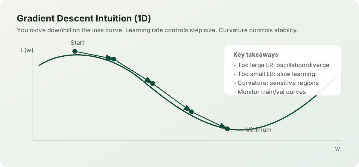
You never fully "see" the loss landscape. You infer direction from noisy gradients. Robust training setups are about controlling instability, not forcing convergence at any cost.

Tradeoffs

• Accuracy vs calibration: high accuracy can still produce bad confidence estimates
• Precision vs recall: fraud detection, moderation, and medical triage require different tradeoff shapes
• Bias reduction vs variance control: more flexibility can learn noise faster
• Fast convergence vs stable convergence: aggressive LR may appear better early and fail late

Details

A) Derive linear regression gradient (practical form)

Given:

• Predictions: y_hat = Xw
• Loss: L(w) = (1/n) * ||Xw - y||^2

Gradient:

• dL/dw = (2/n) * X^T (Xw - y)

Update rule:

• w <- w - lr * dL/dw

What this tells you in practice:

• If feature scales are wildly different, gradient directions become skewed
• Without normalization/standardization, training can oscillate or crawl

B) Regularization from a decision perspective

L2 regularization adds penalty lambda * ||w||^2. Operationally, this discourages brittle coefficients that overreact to noise.

Why this matters for product:

• Improves generalization on unseen cohorts
• Reduces variance and sensitivity to data artifacts
• Often improves stability under minor data drift

C) Confidence intervals and model selection

Suppose Model A beats Model B by 0.4% accuracy. If confidence intervals overlap heavily, shipping A may be unjustified. You need practical significance and risk framing, not just p-values.

D) Loss curves as diagnostic signals

• Train loss down + val loss down: healthy learning
• Train down + val flat/up: overfitting, investigate regularization/data leakage
• Both flat: likely under-capacity, bad features, or optimization issue

Implementation Walkthrough

1. Build synthetic + real small tabular datasets
2. Implement linear regression with NumPy from scratch
3. Train with 3 learning rates (1e-4, 1e-3, 1e-2)
4. Add L2 regularization and compare validation behavior
5. Compute MAE, RMSE, and classification metrics for thresholded outputs
6. Plot calibration curve for one probabilistic classifier
7. Write decision memo selecting one model and one metric contract

Common Failure Modes

• Treating one metric as universally correct
• Interpreting noisy improvement as true signal
• Ignoring class imbalance and calibration
• Using random splits when temporal leakage exists
• Tuning heavily on validation until it becomes training-by-proxy

Interview Depth

Be ready to answer:

• Why choose F1 over ROC-AUC in this product context?
• What training signal indicated overfitting, and what did you change?
• How do you justify model promotion when gains are small and uncertain?
• What regularization choice would you make under mild drift risk, and why?

High-signal response style:

• State assumption
• Explain tradeoff
• Quantify impact
• Propose guardrail

Hands-On Lab

Lab Task

Build an end-to-end notebook called math-foundations-lab.ipynb that includes:

• Linear regression from scratch
• LR schedule experiments
• L2 regularization comparison
• Confidence interval estimation for model deltas
• Metric decision memo section

Required Deliverables

• Plots: train/val loss, residual distribution, calibration
• Table: model variants and metrics
• Written: 1-page recommendation with risk notes

Milestone Checklist

• You can derive and explain gradient updates without copy/paste
• You can identify overfitting from curves and prescribe fixes
• You can justify metrics using product-risk framing
• You can reject statistically weak model improvements confidently
• You can communicate tradeoffs in clear engineering language

Next Step in the Path

Now convert this mathematical reasoning into reproducible engineering execution in Python for ML Workflow (Deep).

---

Diagrams

Workbook

Download and complete:

• /workbooks/math_foundations_workbook.py

Suggested workflow:

1. Run it as-is.
2. Try 3 learning rates.
3. Write 5 bullets explaining what changed and why.

Code Snippets

Here is a minimal NumPy-style reference implementation you should be able to explain line-by-line:

pythonCopy
import numpy as np

X = np.random.randn(200, 3)
y = (X @ np.array([1.2, -0.7, 0.3])) + 0.1 * np.random.randn(200)

w = np.zeros(3)
lr = 1e-2

for step in range(2000):
    y_hat = X @ w
    grad = (2.0 / len(y)) * (X.T @ (y_hat - y))
    w -= lr * grad

Focus questions:

• Why does feature scaling matter for the gradient?
• What would happen if lr is too large?
• How do you decide a stopping criterion without overfitting?